How PitStopper Uses PostGIS to Search Along a Route

When you ask PitStopper to show the cafes, water taps, shops or shelters along a route, it has to answer a question that sounds simple and is not:

Which places are within 500 metres of this 200 km line?

Not near a point. Not inside a box. Along a wiggly line, for 200 km, with the answer arriving before the rider gets bored.

That question has one good answer and several plausible bad ones. We ran one of the bad ones for eight months, and the obvious way to fix it turns out to be another. This post is about how the good one works: what PostGIS is, why the obvious query turns out to be slow, and the small trick that makes the final version fast.

First, what PostGIS is

Three layers, and only the middle one is unfamiliar.

PostgreSQL is an ordinary database, the sort that sits behind most websites. It stores rows of data and lets you search and filter them.

PostGIS is an extension for PostgreSQL that teaches it about shapes. A column can hold a point, a line or an area the same way another column holds a name or a price, and a few hundred new functions let you ask questions about them: what is near what, what crosses what, how far apart two things are.

PitStopper uses the two together to hold a searchable copy of OpenStreetMap, and asks it where things are in relation to your route.

Concretely, a cafe in our database is a row that looks roughly like this:

name      The Coffee House
location  POINT(-0.9016 51.5372)
tags      amenity=cafe

And a route you have loaded is a shape too:

geometry  LINESTRING(-0.89 51.53, -0.91 51.54, ...)

Once both are shapes in the same database, one question becomes askable: which of those points are within 500 metres of that line? That is the whole idea, and everything below is about making it fast.

Where the data comes from

OpenStreetMap is a free map of the world that anyone can edit, the Wikipedia of maps. Over two million people have added the roads, paths, cafes, benches and water taps around them. Everything in it is described with plain key-and-value labels called tags, so a cafe is amenity=cafe and a drinking fountain is amenity=drinking_water, which is what our searches match on.

The part that matters here is that the whole database can be downloaded. We are not asking somebody else's map service politely; we hold our own copy and ask it whatever we like.

The catch is that a copy goes stale, and OSM never stops moving: millions of edits a day, every day. That is why our updates run hourly rather than whenever we remember.

Why not just ask OpenStreetMap?

A fair question, and for a long time that is exactly what we did.

OpenStreetMap is the data. Querying it is a separate problem, and Overpass is the usual answer to it. That is where PitStopper started, and not on somebody else's server either: we ran our own Overpass instance, kept up to date, for eight months.

It worked. It was just slow, and it got slower the longer the route was, because of the shape of the question rather than the shape of the hardware. Overpass answers "what is in this box" well. It can be asked about a line - around: takes a whole polyline, not just a point - but on a route with thousands of points that query is expensive enough to be impractical, and it was cheaper for us to send a lot of boxes instead. So we did: one request each, and then again for every category.

Holding the data ourselves was never the problem. What changed is what we could ask of it. Put the same OpenStreetMap data in PostGIS and the query can be shaped around what PitStopper actually needs, rather than assembled out of the one question the API knows how to answer.

Postpass is the halfway house that showed us this was worth doing. It puts OpenStreetMap into PostGIS and exposes SQL over HTTP: you send it a query rather than parameters, and it hands back GeoJSON, which is a plain text format for describing shapes. No radius=, no fixed set of endpoints, just SQL against a planet-scale mirror. That openness makes a class of question that gives Overpass trouble entirely ordinary.

So the honest lineage of what we run is: Postpass had the idea, we borrowed it, and then wrote our own because we needed less than it offers, not more. Postpass exists to let anyone on the internet run any query. We have one client asking five questions we already know. Almost everything Postpass has to do follows from accepting arbitrary SQL, and none of it is work we need. "From the browser to the database", near the end, is where that difference gets concrete.

Everything starts with a rectangle

A spatial database is fast for one reason. It does not compare your query against every row. It keeps a bounding box for each object, a simple rectangle around it, and the spatial index lets it discard, in a single step, everything whose box does not touch yours. Only the survivors face the exact, expensive geometry test.

That index has a name you will meet in any PostGIS discussion: GiST. It is the one PostGIS builds on a geometry column, and it is what makes "which boxes overlap this box" a single lookup rather than 75 million comparisons. Whenever this post says "the index", that is the one it means.

Very roughly, the index gets to say: this cafe is obviously nowhere near the area we care about, so ignore it.

So the size of your box decides everything.

Ask "what is within 500 m of this cafe" and your box is a square a kilometre across. The index throws away the planet and hands back forty candidates. Ask "what is within 500 m of this 200 km route" and your box is the smallest rectangle containing the entire route, which is a county or two. The index throws away nothing, and every point in the database goes through the exact test one at a time.

That one fact explains both the approach we shipped and the query you would naturally write to replace it.

What we shipped first: boxes all the way down

Cover the route in a chain of bounding boxes and query each one. That is what those eight months were. It works, and it wastes a great deal, because a box round a diagonal stretch of road is mostly fields and a route that bends needs a lot of boxes. Overpass also responds badly to a single query carrying fourteen unrelated tag filters, so it was boxes times categories, and a long ride became dozens of requests, several of which timed out.

Worth being clear about where the time went, because it was not the server. Our instance was ours, it was kept up to date, and it was not fighting anyone else for capacity. The cost was in the shape of the question: dozens of round trips per search, each one handing back things the rider would never pass.

The corridor is the shape you actually mean

We do not really want to search a rectangle. We do not want to search a hundred little rectangles either.

What we actually mean is: give me everything inside this band following the route.

That is a corridor. If the route is 200 km long and the search radius is 500 metres, the corridor is simply the route with 500 metres added either side. PostGIS will draw that shape for us, with a function called ST_Buffer.

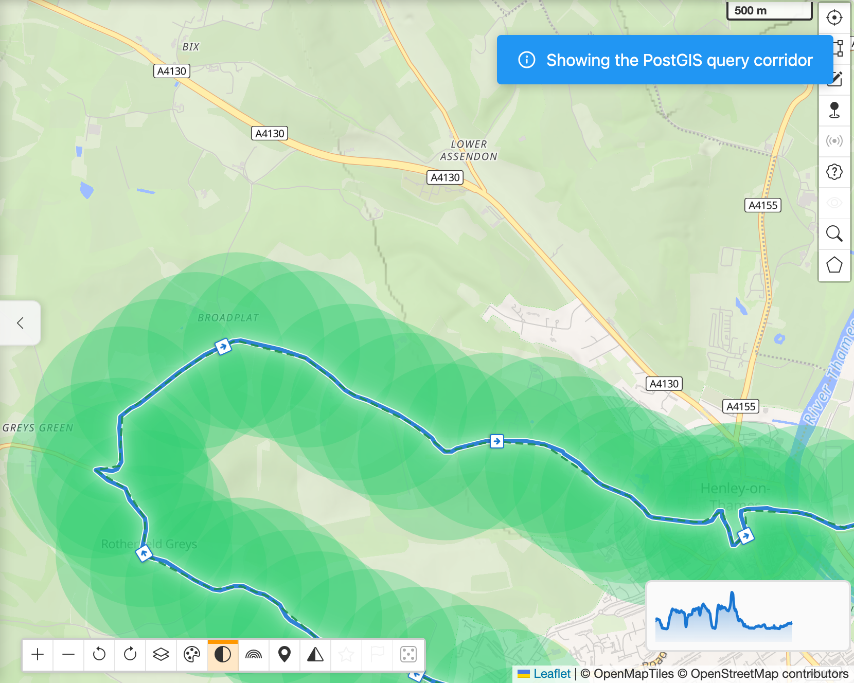
The important thing is that this is not an approximation of the route. It is the search area we actually mean. Here is one, drawn by the app at the radius the query really uses:

And the same view after the search, showing the points that corridor returned:

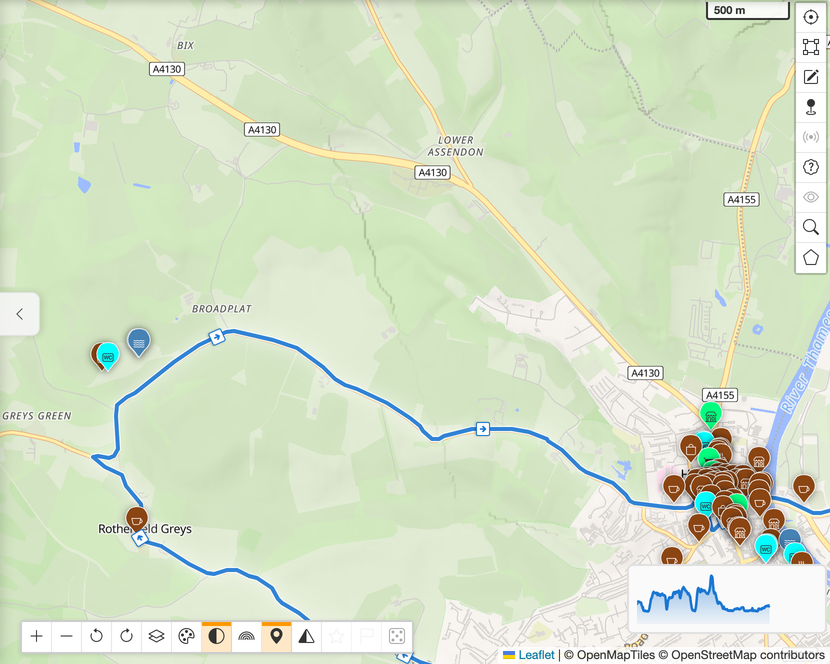
The cluster in Henley is what you would expect. The pair out at Broadplat is the interesting one: several hundred metres off the road, nothing around them, exactly what a careless "close to the route" test throws away. It is also the only water for eight kilometres.

The query you write first

Move to PostGIS and the corridor stops being a shape you have to approximate with boxes. You can simply ask for it:

SELECT * FROM pois
WHERE ST_DWithin(geom::geography, route::geography, 500);

In English: give me every place that is within 500 metres of this route.

If SQL is not your language, the parts are:

• pois is our table of places, one row per cafe, tap, bench or shelter. 75 million of them.
• geom is where a place is, and route is the line you loaded.
• ST_DWithin is the question: are these two shapes within 500 of each other? Almost every PostGIS function is named ST_ something, for "spatial type". (GeometryType and postgis_version are among the few that are not.)
• ::geography is what makes the 500 mean 500 metres rather than 500 degrees. It matters more than it looks, and there is a section at the end for anyone who wants that story.

Correct, readable, and on a long route it is a table scan wearing a spatial index's clothes. "Every place we hold" is 75 million distance calculations against a 200 km line.

Two things are wrong with it, and the second is the one this post is about. The immediate problem is that ::geography: converting a column on the way past means the index built on that column cannot be probed at all, so the query never reaches the rectangle stage. Fix that, and you meet the rectangle - the box round a 200 km line still hands over most of the database for the exact test to grind through. The cast is a mistake you can correct in a minute; the rectangle is the shape of the problem. The planner section below has the receipts for both.

The fix: chop the band into tiles

A 200 km corridor is itself an enormous shape, and the box around it is the same county or two as before. So we cut it into short sections, using ST_Subdivide.

Think of it as handing the database a map made of small tiles instead of one enormous sheet. Each tile is small, so the rectangle around it is small, so the index is useful again: for every tile it can throw away almost the entire database in one step. Same answer, found for a fraction of the work.

The distinction worth holding on to is that we split the corridor for the database's benefit, not because we are approximating the route. The band is still the band.

Didn't we already do this with bounding boxes?

Said quickly, the two approaches sound like the same idea twice: cut the route up, ask about each piece. The difference is what the pieces are, and who ever sees them.

Boxes, over Overpass	Corridor cells, inside PostGIS
Boxes are thrown over the route	The corridor already follows the route
The box is the question	The cell is how the index is asked the question
Sent over the network, one request each	Never leave the database
Whatever is in the box comes back	Candidates are tested against the real band first
A cafe three fields away is a result	A cafe three fields away is dropped before the answer is sent
Dozens of requests, some timing out	One request, every category at once

The Overpass boxes were the question. A rectangle went out over the network and whatever was inside it came back. A cafe in the corner of a box, three kilometres from the road, arrived, was counted, and the app had to work out for itself that you would never pass it. Because a rectangle over a diagonal road is mostly fields, that happened constantly.

The corridor cells are plumbing you never see. Each cell turns up a handful of candidates, every candidate is then tested against the corridor's real shape, and anything not genuinely within 500 m of the road is dropped before the answer leaves the database.

So the shape of the question went from a chain of rectangles near the route, which is an approximation, to the corridor itself, which is the actual thing you meant. The chopping stayed; what got chopped, and what came back, both changed.

What actually happens when you search

your route
    |  thinned to a few hundred points
    v
sent as GeoJSON
    |  ST_Buffer, 500 m
    v
a corridor
    |  ST_Subdivide
    v
short sections
    |  spatial index, one step per section
    v
candidate places
    |  tested against the real corridor, then the tag filters
    v
results

What this means for a rider

Go back to those two taps at Broadplat.

They sit a few hundred metres off the road, with nothing else around them, and they are the only water for eight kilometres. A box drawn near the route might catch them or might not, depending on where the box happened to end. A "close to the route" test that measures to the nearest recorded point can put them just outside. They are exactly the kind of thing that gets quietly dropped, and they are also the one result on that map a rider would actually have wanted.

Asking the real question - everything inside a band 500 metres either side of the line I am riding - is how you get them back. That is what all of this is for. The rest is what it makes possible:

• Long routes no longer mean hundreds of separate searches.
• Every category is searched together rather than one request each.
• The search area follows the route instead of being a collection of large boxes near it.
• The filtering happens in the database, so what crosses the network is the answer rather than the raw material.
• The same approach works for a 20 km evening loop and a 700 km tour.

Ask for everything within 500 metres of a 700 km route and that is one question, asked once.

The numbers. Two runs on the same day, 11 July 2026, from the harness in the repo (tests/e2e/poi-backend-compare.diag.spec.js) against staging. It matters which is which.

The first is the one that justified the move. It put the old Overpass path against a PostGIS corridor query, cold both sides:

the search	Overpass	PostGIS corridor
6 km, 8 categories	4.3 s	0.19 s
180 km, 8 categories	9.7 s	0.66 s
180 km, 20 categories at 1 km	20.1 s	0.85 s
700 km, 8 categories	never finished, 120 s timeout	2.8 s
700 km, 20 categories at 1 km	never finished, 120 s timeout	4.1 s

Fifteen to twenty-four times faster on the searches that finished, and two that stopped being failures. The PostGIS column there is Geofabrik's public Postpass, because at that point we had not built anything of our own. (The full table in the repo has nine rows and a wider spread, from 3x on a dense 5 km point search to 34x on a short route with twenty categories.)

Later the same evening, once our own server existed, a second run put all three side by side. Our node beat the public instance on every row, which is the argument for running your own: same idea, but the questions are fixed in advance and the data is filtered to what we actually ask for.

the search	public Postpass	our own server
6 km, 1 category	157 ms	79 ms
180 km, 1 category	909 ms	182 ms
180 km, 8 categories	685 ms	241 ms
180 km, 20 categories at 1 km	933 ms	312 ms
parking at 170 m, Reading	8 s timeout	206 ms

Two rows there need a caveat rather than a boast.

One category on the 180 km route came back slower than eight on the same route, which cannot be true of the work being done. The public instance is a free shared service with no response cache, so its numbers move with whatever everyone else is asking it at that moment. Read that column as an order of magnitude and nothing finer. The noise is part of the argument for running your own; it is not evidence that we are four times better at this.

The parking row is not a Postpass bug either, and it is the most useful line in the table. amenity=parking is one of the largest tag sets in OpenStreetMap: we hold 6.8 million of them, and simply counting them all takes half a minute. The answer to "parking within 170 metres of this point in Reading" is two. Everything rests on discarding the other 6,767,260 by rectangle before anything looks at a tag, which is the subject of this whole post, and exactly what the ::geography cast quietly prevents.

Two runs on one day, so read all of it as orders of magnitude rather than benchmarks. The shape is what matters: the search stopped scaling with the length of the route.

The band is real metres wide

Because the band is drawn in metres rather than degrees, its width is true at any latitude, and the debug overlay draws it the same way. What you see on the map is the query.

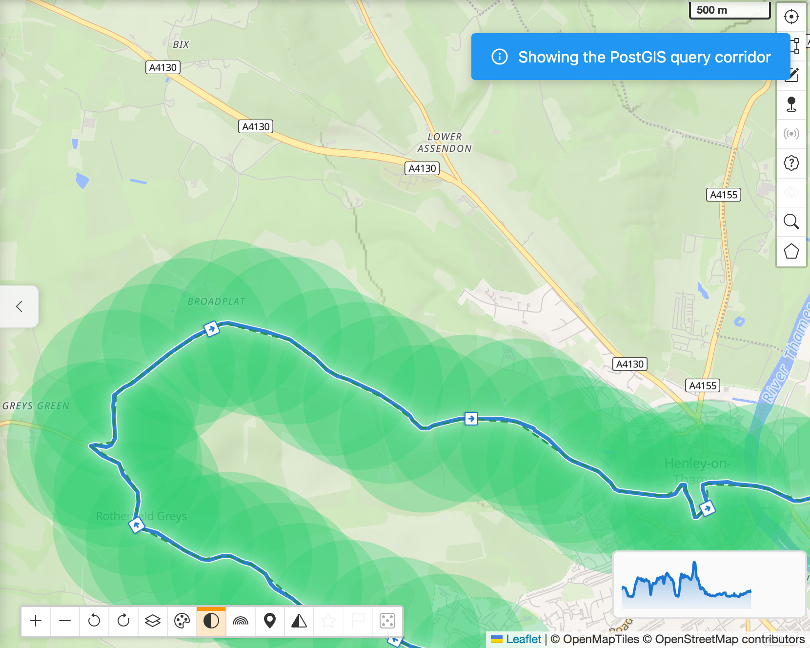
That is the same view at 100 m rather than 500 m. Nothing about the query changes but the number.

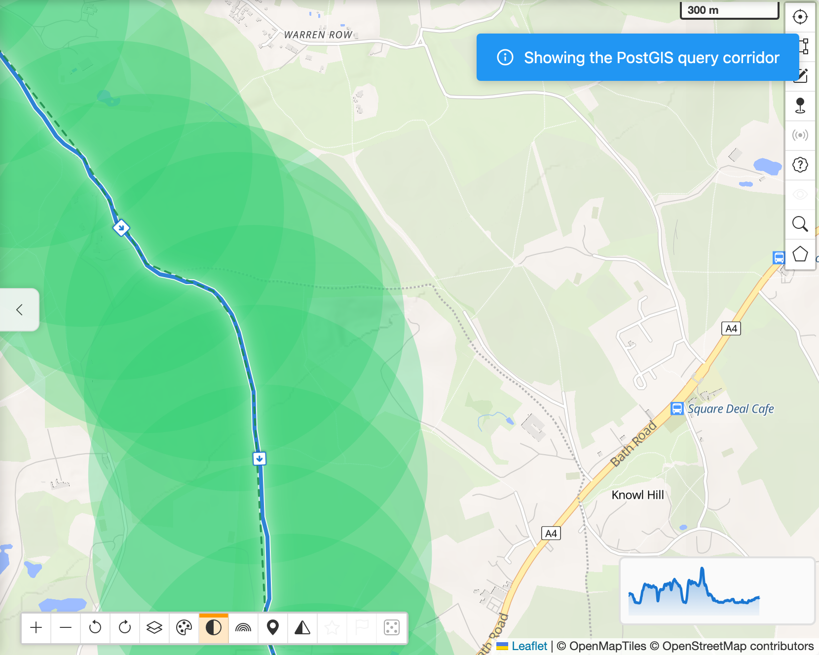
The same overlay on a bend. The edge of the band holds the same distance from the road all the way round the curve, which is what "within 500 metres of the route" actually means. Everything east of it here is simply not in the question: the fields, Knowl Hill, the A4 through it.

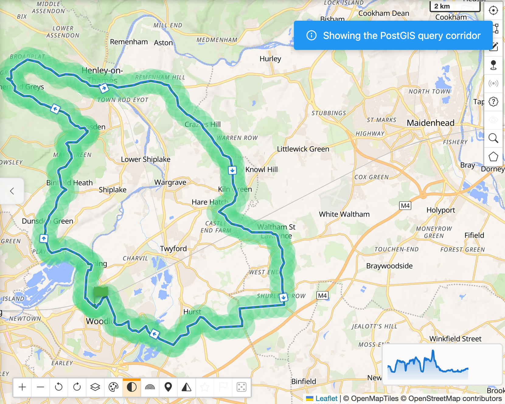
The whole 44 km ride. One request.

Before the request leaves the browser

Most of the route's points are thrown away first. A recorded GPX holds ten thousand of them; the corridor needs a few hundred. Douglas-Peucker at a 25 m tolerance does the thinning, and it cuts the request body by an order of magnitude. The trade is exact and worth stating: the thinned line stays within 25 m of the recorded one, so the edge of the corridor can move by up to 25 m. A tap 490 m from the track you rode can come back 515 m from the line we sent. At a 500 m radius nobody notices; at 100 m it is a quarter of the width, which is the radius to keep it in mind at. The overlay draws the thinned line, so the picture stays honest about what was actually sent.

A cap of 10,000 points and a 35 km radius, enforced on the server. Nobody asks for more. We would just rather find the limit ourselves than have a rider find it on a Sunday morning.

Counting without fetching

Sometimes you want to know what is ahead before fetching any of it: 84 cafes, 2 water taps, no fuel for 60 km. The app can say so up front, and you can then decide what is worth asking for.

That is the same corridor asked to count rather than return:

SELECT cat.key,
       count(*) FILTER (WHERE poi_matches_filters(cand.tags, cat.value))
FROM jsonb_each(categories) AS cat(key, value)
LEFT JOIN candidates cand ON true
GROUP BY cat.key;

It hands back no points at all, only numbers, which is exactly the point: a cap on how many rows may come back cannot quietly spoil a count when no rows come back. Categories with nothing along the route return zero rather than going missing, because "none here" and "we did not check" are different answers and the UI says which one it has.

For the SQL-curious

Everything above is the idea. This is the query, and the three things we got wrong before we got them right.

CREATE OR REPLACE FUNCTION pois_along_route(
    route_geojson TEXT, radius_m INTEGER, filters JSONB
) RETURNS TABLE (...) LANGUAGE sql STABLE PARALLEL SAFE AS $
    WITH corridor AS (
        SELECT ST_Subdivide(
            ST_Buffer(
                ST_SetSRID(ST_GeomFromGeoJSON(route_geojson), 4326)::geography,
                radius_m
            )::geometry,
            64) AS cell
    ),
    candidates AS (
        SELECT DISTINCT p.osm_type, p.osm_id, p.geom, p.tags, p.osm_timestamp
        FROM pois p
        JOIN corridor c ON p.geom && c.cell AND ST_Intersects(p.geom, c.cell)
    )
    SELECT osm_type, osm_id, ST_Y(geom), ST_X(geom), tags, osm_timestamp
    FROM candidates
    WHERE poi_matches_filters(tags, filters);
$;

4326 is ordinary lat/lon. Every coordinate system has a number, and 4326 is the one the whole world uses for degrees of latitude and longitude: it is what a GPS reports and what sits in a GPX file. ST_SetSRID tells PostGIS that is what the incoming numbers are, because GeoJSON carries the coordinates but not the system.

Buffer in metres, compare in degrees. The band has to be drawn in metres, because the radius is metres and the import is planet-wide: a degree-based buffer set for Oxfordshire comes out barely half as wide east to west in Tromsø, as the two bands in the diagram above show. North to south it is unchanged, a degree of latitude being the same length everywhere, so what you actually get is not a narrower band but a squashed one. But the comparison has to be geometry against geometry, or the index does not apply. So draw the band in geography, convert the result back, and compare in geometry.

::geography is a cast - SQL for converting a value from one type to another - and it is the same one in the simple query near the top, doing the job the Tromsø diagram shows.

Chopping the band up is the whole trick. A buffered 200 km corridor is one enormous polygon with the same useless bounding box, so testing against it is no better than the naive version was. ST_Subdivide into cells of at most 64 vertices gives dozens of small polygons with tight boxes. In database terms: it is what lets PostgreSQL's query planner use a bitmap index scan per cell instead of reading the table from front to back.

Remove the duplicates, because the sections touch. A cafe sitting exactly on the join between two sections is found twice. One DISTINCT: cheap to fix, silly to ship without.

Asking the planner to show its working

SQL says what you want, never how to get it, so something has to decide the how: that is the planner. Given a query it works out the possible ways to answer it, guesses what each would cost, and runs the cheapest. Using an index is one of those ways, and the planner will only take it if it can see how; otherwise it reads the table from front to back, which is called a sequential scan.

The ::geography conversion breaks that twice over. The geom column is geometry-typed, so converting it means the index built on it cannot be used at all: the planner has nothing to probe. And even if it could probe, we are back to the rectangle, where the box round a 200 km line hands over a million candidates anyway.

You can ask the planner to show its working, with EXPLAIN, and it is blunt about this one. It puts a cost on each way of answering: an estimate of how much work that plan would take. Lower is better. The number is internal, not seconds, so one on its own tells you nothing, but two side by side tell you plenty.

For the simpler version of this query, a circle round one cafe where the same conversion defeats the same index in the same way:

How it plans to answer	Estimated cost (lower is better)
Read all 75 million rows and measure each one	4,500,000,000
Check the boxes first, then measure the survivors	4,600

Same question, same data, same answer at the end. The planner expects one of them to be about a million times more work than the other, which is its way of telling you it has given up on your index.

From the browser to the database

Everything so far has been about the shape of the query, right down to the SQL. This last piece is about who writes it, which turns out to be the bigger difference between what we run and the thing it is modelled on.

The browser never sends SQL.

What leaves the browser is a JSON object with four fields:

{
  "mode": "route",
  "route": [[[51.54, -0.90], [51.53, -0.92], ...]],
  "radius_m": 500,
  "filters": [[{"k": "amenity", "v": "cafe"}],
              [{"k": "amenity", "v": "drinking_water"}]]
}

route is the thinned line from "Before the request leaves the browser". filters is the category list, one group per thing you ticked. There is no query in there, only four values.

nginx is the web server sitting in front of ours. It terminates TLS (the s in https) and does the unglamorous work: the Origin header has to be a pitstopper.net host, three requests a second with a burst of fifteen, a 2 MB body cap. Then it keeps a response cache keyed on the request body, which is only possible because the body has a fixed shape. Two riders asking for the same categories along the same corridor share one trip to the database.

That cache is allowed to hold an answer for 24 hours, which sounds like it contradicts the hourly updates. It does not, because every hourly update empties it as its last step. The 24 hours is a ceiling that is never reached: a repeated search is at most one update behind, and the per-category reload button sends ?nocache=1 to skip the cache entirely.

server.js checks the shape and the limits, and that is honestly all it does. Mode is route or point. Radius between 25 m and 35 km. At most 10,000 points across at most 32 routes; at most 128 filter groups of at most 8 tag pairs; no tag longer than 256 characters. Then it turns [lat, lon] into GeoJSON's [lon, lat] and makes one call:

pool.query('SELECT * FROM pois_along_route($1, $2, $3::jsonb)',
           [geojson, radius, filters]);

Those are bound parameters rather than string concatenation. The statement is a constant sitting in the file and the values travel beside it, never pasted into it, so there is nothing a cleverly-named tag could smuggle in: no way to end the query early and start a new one of your own. That trick is SQL injection, and it has been emptying databases since the nineties.

PostGIS then does everything the rest of this post is about. The five functions in schema.sql are the whole query surface: pois_along_route, pois_around_point, pois_count_by_category, ways_along_route and ways_around_point.

Because the shim holds nothing, it could be PostgREST or pg_featureserv instead and neither the client nor the SQL would notice. That is not tidiness for its own sake. It is what let us run the whole backend against the old Overpass path in production, same client and same categories behind a flag, and get numbers instead of opinions.

Which is not how Postpass works, on purpose

Postpass takes SQL. You POST it a statement, it runs it, you get GeoJSON back. That is the point of it, and it is exactly why it was the right thing to prototype against: we could try a corridor query against a planet-scale mirror without deploying anything at all.

We still use it, and not as a museum piece. Geofabrik's public instance is the tier we fall to when both of our own nodes fail, and since the Overpass fan-out was deleted in August 2026 there is nothing behind it: Postpass is the last thing standing between a rider and no answer at all.

So both shapes in that picture are live in the same browser. If our server answers, the client sent parameters. If it does not, the same client builds a SELECT and posts it to Geofabrik. One search, two completely different ideas about who writes the query, chosen at runtime by whether our hardware is up.

The trade is worth being plain about.

What we give up is generality. Any question we did not think of in advance needs a new function and a deploy, where a Postpass user would just write a different SELECT.

What we get back only works when the shape is known in advance. The planner sees the same five statements forever, so a plan can be checked once and then trusted, instead of being worked out at request time from whatever SQL turned up. The response cache can key on the body. And the limits above are enforceable, because "at most 10,000 points" is something you can say about a field and not something you can say about a query.

What it costs to run

Measured on 12 September 2026 on one of our two nodes - srv01, which answers requests as poi01 - running a planet import with our tag allowlist. Not estimated, and bigger than you might expect from a post about points of interest, for a reason worth seeing.

POI rows	75.7 M
Way rows	266 M
Database on disk, indexes included	219 GB
osm2pgsql flat-nodes store	106 GB
Filtered planet PBF	33 GB
Node server, memory in use	49 MB

The database breaks down about like this: ways is 102 GB, osm2pgsql's own planet_osm_ways middle table another 91 GB, and pois (the table this whole post is about) only 24 GB. The POI half is the cheap half. Full road geometry is what costs, and we bought it deliberately, for the three features a centroid cannot serve.

The flat-nodes store is not in the database at all: it is a flat array on disk indexed by OSM node id, which is how osm2pgsql avoids holding the planet's node positions in RAM. It costs 106 GB of permanent disk to save roughly that much memory. Put it on your fastest drive. We once moved ours onto a USB NVMe by accident and hourly updates went from 33 seconds to 17 minutes.

Import is osm2pgsql in flex mode against a generated allowlist, in two halves: wide keys taken at any value (amenity, shop, tourism, leisure, historic, emergency, office, healthcare, craft), and exact pairs for keys where taking the bare key would import half the planet's geometry rather than its points of interest.

A way lands in both tables. pois holds its centroid, which is right for a cafe inside a building, and ways holds its full geometry, which is the only thing that can answer "where does the surface change" or "snap this point to a road". A centroid cannot draw a tunnel.

Updates run hourly; a full rebuild from planet runs monthly. The provenance row carries both timestamps, because "how old is the foundation" and "how old is the newest change" are different questions, and a staleness watchdog needs the first one.

If you are running Postpass

Postpass is deliberately general: send it any SQL you like. We wanted the opposite: five functions answering five fixed questions, with the plan for each settled in advance rather than decided at request time by whatever SQL somebody sent us. Less flexible on purpose, and predictable because of it.

To be clear about what we did and did not take: the idea is Postpass's, the code is not. We run no Postpass, and our server is not a fork of one. What we copied was the recipe anyone can copy - osm2pgsql into PostGIS, HTTP in front - and then wrote roughly two hundred lines to serve the five questions we actually ask. If you need the general thing, run Postpass. It is good, and writing your own is only worth it when your requirements are narrower than the project's, which is a smaller set of people than it sounds.

If you want route corridors on your own instance, take ST_Subdivide on a geography buffer and leave the rest. That one call is the difference between a query that reads correctly and a query that runs. Everything else here is our particular taste in tag filters.

One other transfer is worth an hour of your time if you are migrating off Overpass rather than starting fresh: our response shape is deliberately Overpass-compatible, {elements: [...]} with raw tags, nodes carrying lat/lon and ways a centre point. The client that spoke to Overpass needed an adapter and about an afternoon.

Seeing the corridor for yourself

Everything pictured above is System → Show Search Area in PitStopper, on any loaded route. It draws metre-true circles along the thinned line at the live radius, so dragging the radius slider redraws the real query area. We built it to debug this work and left it in, because a spatial query you cannot see is a spatial query you are guessing about.